- About the Course:
This course provides a broad introduction to the field of nonlinear dynamics, focusing both on the mathematics and the computational tools that are so important in the study of chaotic systems. The course is aimed at students who have had at least one semester of college-level calculus and physics, and who can program in at least one high-level language (C, Java, Matlab, R, ...)
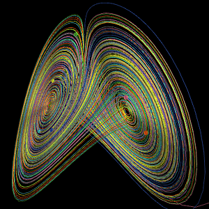
After a quick overview of the field and its history, we review the basic background that students need in order to succeed in this course. We then dig deeper into the dynamics of maps—discrete-time dynamical systems—encountering and unpacking the notions of state space, trajectories, attractors and basins of attraction, stability and instability, bifurcations, and the Feigenbaum number. We then move to the study of flows, where we revisit many of the same notions in the context of continuous-time dynamical systems. Since chaotic systems cannot, by definition, be solved in closed form, we spend some time thinking about how to solve them numerically, and learning what challenges arise in that process. We then learn about techniques and tools for applying all of this theory to real-world data and close with a number of interesting applications: control of chaos, prediction of chaotic systems, chaos in the solar system, and uses of chaos in music and dance.
In each unit of this course, students will begin with paper-and-pencil exercises regarding the corresponding topics, and then write computer programs that operationalize the associated mathematical algorithms. This will not require expert programming skill, but you should be comfortable translating basic mathematical ideas into code. Any computer language that supports simple plotting—points on labelled axes—will suffice for these exercises. We will not ask you to turn in your code, but simply report and analyze the results that your code produces.
- About the Instructor(s):
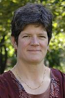
Elizabeth Bradley did her undergraduate and graduate work at MIT, interrupted by a one-year leave of absence to row in the 1988 Olympic Games, and has been with the Department of Computer Science at the University of Colorado at Boulder since January of 1993. Her research interests include nonlinear dynamics, artificial intelligence, and control theory. She is the recipient of a NSF National Young Investigator award, a Packard Fellowship, a Radcliffe Fellowship, and the 1999 student-voted University of Colorado College of Engineering teaching award.

Angela Stewart is a fourth year PhD student at the University of Colorado Boulder. Her research is in using artificial intelligence and machine learning techniques to improve education. She is particularly interested in modeling complex student behaviors to help them learn better. Angela is very excited to be TAing the course and looks forward to virtually meeting all the students.
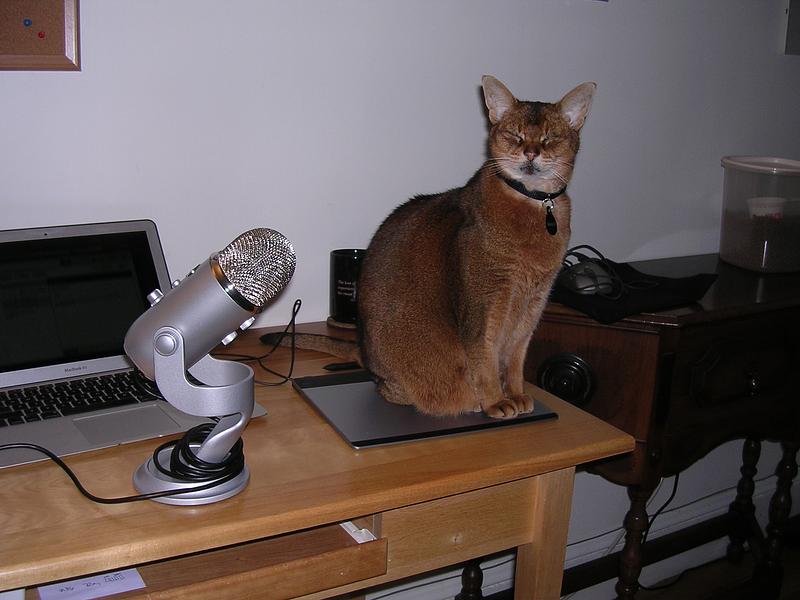
- Course Team:
Videography assistant: Gabriel (helpfully sitting on the tablet that Liz uses during videos)
- Class Introduction:
- Class Introduction
- How to use Complexity Explorer:
- How to use Complexity Explorer
- Enrolled students:
-
1,561
- Course dates:
-
15 Jan 2019 3pm UTC to
15 May 2019 5pm UTC - Prerequisites:
-
Calculus (derivatives), physics (introductory classical mechanics), and computer programming skills (language of your choice).
- Like this course?
- Donate to help fund more like it
- Twitter link
Syllabus
- Introduction and Maps I
- Maps II
- Flows I
- Flows II
- Flows III
- Flows IV
- Flows V
- Nonlinear time-series analysis I
- Nonlinear time-series analysis II
- Applications